Elbow Method for k-means

Performance Metric: SSE

In the previous implementation of k-means++, when comparing it with plain k-means, success or failure was heuristically judged based on the following criteria:

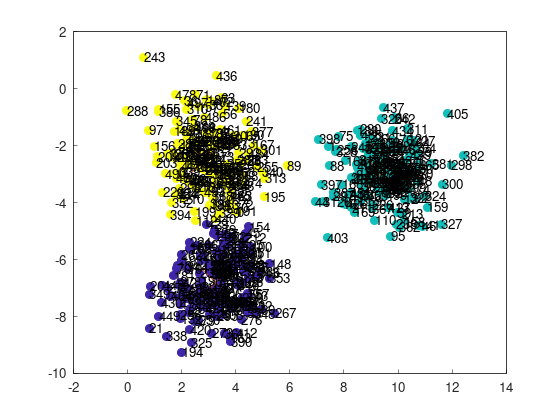
• The 243rd point in the upper left and the 21st point in the lower left were classified into different clusters => Success
• The 243rd point in the upper left and the 21st point in the lower left were classified into the same cluster => Failure

However, a better method exists.

For each k-means result, a metric called SSE (Sum of Squared Errors) is calculated to evaluate the “goodness of fit.”

SSE is computed by summing the squared distances between each data point and its assigned cluster centroid.

If clustering works well, the distance between each point and its centroid will be small, resulting in a smaller SSE. Conversely, poor clustering leads to a larger SSE.

Fundamentally, k-means can be seen as an algorithm that minimizes (optimizes) SSE through label and centroid updates, making SSE a natural choice for evaluation.

We can add an sse field to the previously implemented KMeans class and update it within the update_labels() function:

sse = 0;
for (int i = 0; i < m; ++i)
{
    double min_dist = std::numeric_limits<double>::max();
    int min_label = -1;
    for (int j = 0; j < k; ++j)
    {
        double dist = distance(points[i], centroids[j]);
        if (dist < min_dist)
        {
            min_dist = dist;
            min_label = j;
        }
    }
    if (labels[i] != min_label)
    {
        updated = true;
        labels[i] = min_label;
    }
    sse += min_dist * min_dist;
}

In scikit-learn’s KMeans class, SSE can be accessed via the inertia_ field, described officially as follows:

inertia_: float

Sum of squared distances of samples to their closest cluster center, weighted by the sample weights if provided.

Running k-means Multiple Times to Select the Best Result

In the previous experiment, applying k-means++ to a dataset improved the success rate from 82.2% to 92.7%.

However, a failure rate of 7.3% might not be acceptable depending on the situation.

To address this, we can repeatedly execute k-means++ with different initializations and select the result with the smallest SSE.

If the success probability for one run is $p$, then the success probability after $n$ runs, $p_n$, is given as the complement of the probability of $n$ consecutive failures:

$$ p_n = 1 - (1 - p)^n $$

For $p = 0.927$:

$$ p_2 = 0.994671 $$

$$ p_3 = 0.999610983 $$

$$ p_4 = 0.999971601759 $$

$$ p_5 = 0.999997926928407 $$

This results in a dramatic improvement.

Let’s add a function to implement this approach:

// Execute k-means++ n times and return the result with the best SSE
template <KMeansablePoint Point>
std::unique_ptr<KMeans<Point>> kmeans_plus_plus_multi(int n, int k, int max_iter, const std::vector<Point> &points)
{
    auto kmeans_opt = std::make_unique<KMeans<Point>>(k, max_iter, points);
    kmeans_opt->sse = std::numeric_limits<double>::max();

    auto kmeans_exc = std::make_unique<KMeans<Point>>(k, max_iter, points);

    for (int i = 0; i < n; ++i)
    {
        kmeans_exc->exec_kmeans_plus_plus();
        if (kmeans_exc->sse < kmeans_opt->sse)
        {
            kmeans_opt.swap(kmeans_exc);
        }
    }

    return kmeans_opt;
}

Here, std::unique_ptr::swap is used to minimize copying.

Using SSE to Determine the Number of Clusters

The need to predefine the number of clusters k is a downside of k-means, but the SSE metric can help determine the optimal cluster count.

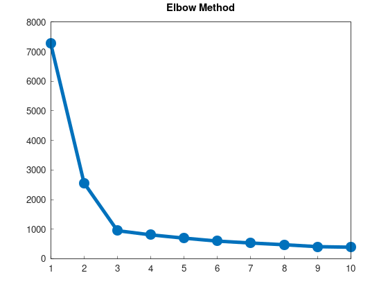
By running k-means with varying k, plotting SSE changes, and identifying where the decrease in SSE levels off, we can estimate the optimal k.

When the number of clusters equals or exceeds the number of data points, each data point forms its own cluster, resulting in an SSE of 0.

SSE decreases monotonically with increasing k, but at some point, the rate of decrease slows, forming a point resembling an “elbow.”

This point is considered the optimal number of clusters.

This method is widely known as the Elbow Method due to the resemblance to an elbow.

An implementation to plot k vs. SSE is provided in example/example_kmeans_elbow_blobs_2d.cpp:

int main()
{
	std::vector<double> sses(10);
	std::vector<double> ks(10);
	for (int k = 1; k <= 10; ++k)
	{
		auto kmeans = yhok::cluster::kmeans_plus_plus_multi(5, k, 100, dataset_blobs_2d);
		sses[k - 1] = kmeans->sse;
		ks[k - 1] = k;
	}
	matplot::plot(sses);
	matplot::title("Elbow Method");
	matplot::show();

	return 0;
}

The result confirms the presence of an “elbow,” suggesting k = 3 as the optimal number of clusters for this dataset.

• Programming
• C++
• Machine Learning