Fresnel Integrals

What are Fresnel Integrals?

Fresnel integrals are two functions defined by the following integrals:

$$S(x)={\int }_0^x\sin (t^2)dt$$

$$C(x)={\int }_0^x\cos (t^2)dt$$

While these are the most common definitions, another set of definitions involving a constant factor is also used:

$$S(x)={\int }_0^x\sin (\frac{\pi }{2}{t}^2)dt$$

$$C(x)={\int }_0^x\cos (\frac{\pi }{2}{t}^2)dt$$

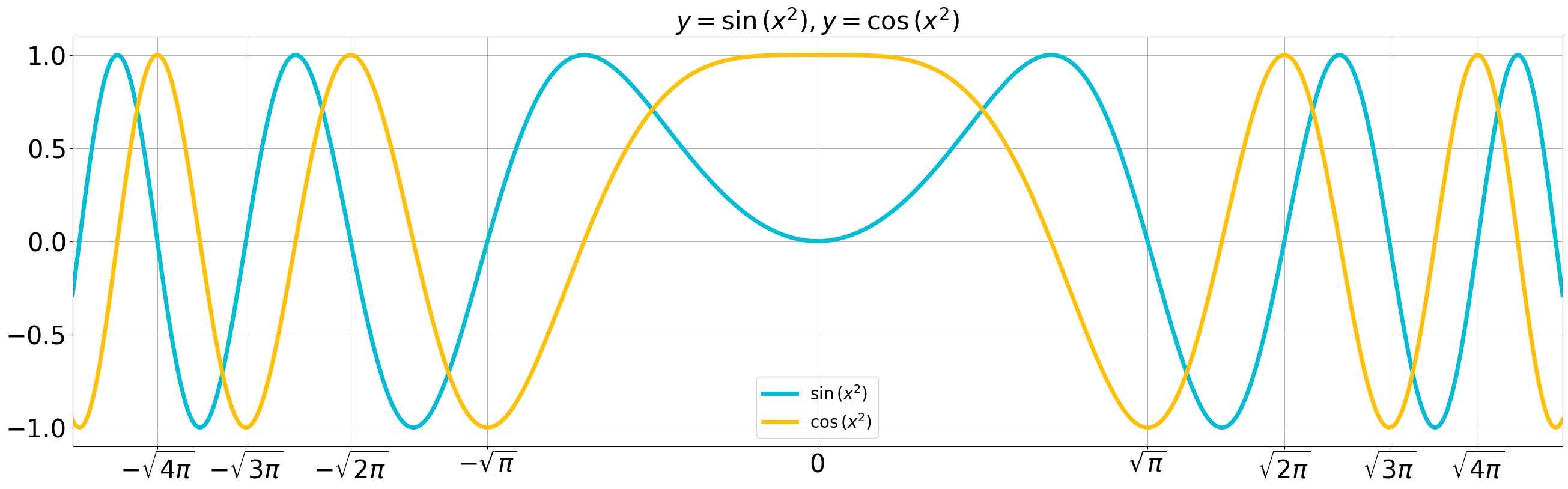
Graphs of $\sin (x^2)$ and $\cos (x^2)$

First, let’s examine the behavior of the integrands $\sin (x^2)$ and $\cos (x^2)$.

Both are even functions and appear smooth near zero, but their oscillations become more intense (i.e., their periods shorten) as they approach the ends.

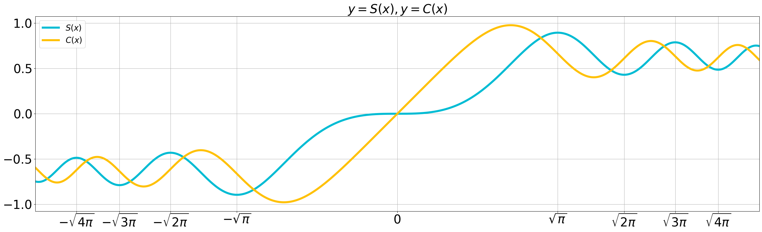
Graphs of $S(x)$ and $C(x)$

Next, let’s visualize the Fresnel integrals $S(x)$ and $C(x)$.

Both are odd functions and are bounded.

They oscillate at both ends, but the amplitude of these oscillations decreases gradually, suggesting that they converge as $x\to \mathrm{\infty }$.

Graphs of $(C(t),S(t))$

Let’s also consider the trajectory when $x=C(t)$ and $y=S(t)$.

As $t\to \pm \mathrm{\infty }$, the trajectory is believed to spiral infinitely while converging to a single point.

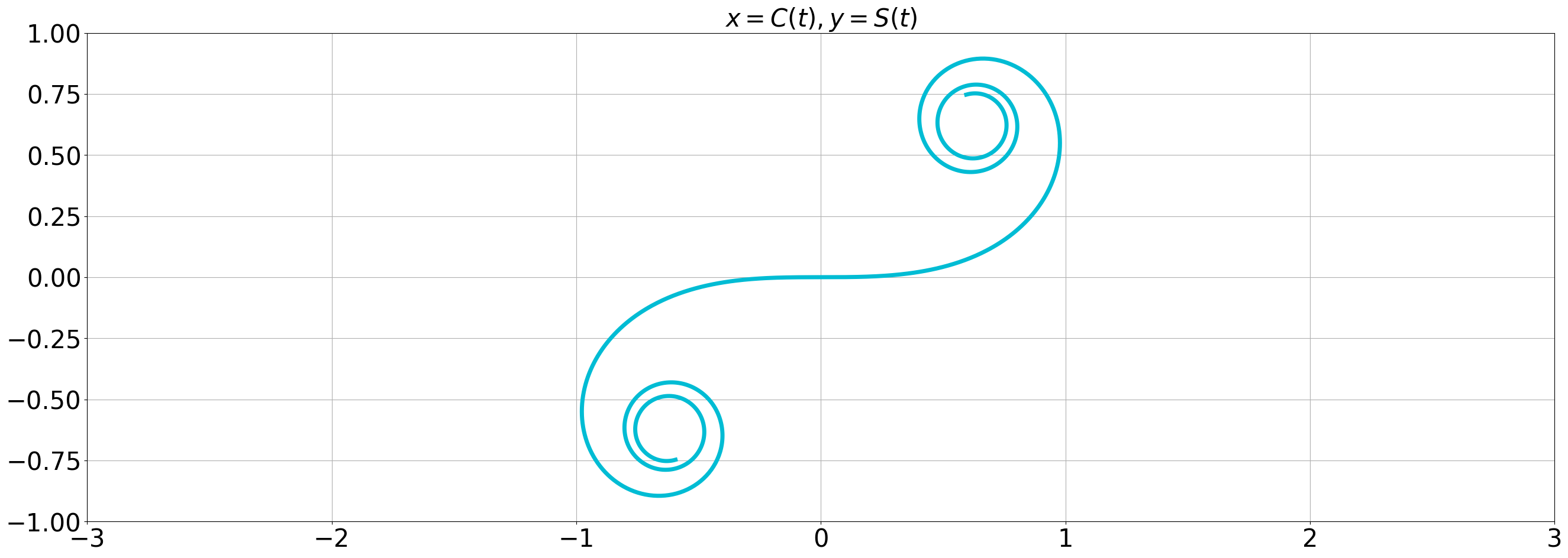
This trajectory is called the Euler spiral, also known as the clothoid or Cornu spiral.

The name “clothoid” was given by Cesàro in honor of the Greek goddess Clotho, who is symbolized by a spool.

Fresnel Integrals in SciPy

The above graphs were created using the scipy.special.fresnel function from the SciPy library.

This function implements the second set of definitions mentioned earlier.

https://docs.scipy.org/doc/scipy/reference/generated/scipy.special.fresnel.html

The graphs above were generated with some suitable transformations.

Limits of Fresnel Integrals

As suggested by the graphs, Fresnel integrals converge as $x\to \mathrm{\infty }$. Let’s determine this limit.

Consider

$${\int }_0^{\mathrm{\infty }}\sin (t^2)dt$$

$${\int }_0^{\mathrm{\infty }}\cos (t^2)dt$$

Instead of evaluating these integrals individually, consider:

$${\int }_0^{\mathrm{\infty }}\{\cos (t^2)+i\sin (t^2)\}dt={\int }_0^{\mathrm{\infty }}{e}^{i{t}^2}dt$$

Textbook Solution

Let $R$ be a positive real number, and consider the following contour integration path:

$$C_1:0\to R$$

$$C_2:R\to R\exp [\frac{\pi }{4}i]$$

$$C_3:R\exp [\frac{\pi }{4}i]\to 0$$

$$C=C_1+C_2+C_3$$

Here, $C_1$ is a straight path along the real axis, $C_2$ is a circular arc of one-eighth of a turn, and $C_3$ is a straight path back to the origin.

We denote the complex integrals along each path as $I_1$, $I_2$, and $I_3$, respectively, and aim to find the limit of $I_1$ as $R\to \mathrm{\infty }$.

Since $e^{i{z}^2}$ is analytic and $C$ is a simple closed curve in the complex plane, by Cauchy’s integral theorem,

$$I=I_1+I_2+I_3=0$$

Let’s calculate $I_2$ and $I_3$. To summarize, $I_2$ converges to $0$, and $I_3$ becomes a Gaussian integral.

$$I_2={\int }_{C_2}{e}^{i{z}^2}dz={\int }_{\theta =0}^{\frac{\pi }{4}}\exp [i(R{e}^{i\theta }{)}^2]\cdot iR{e}^{i\theta }d\theta$$

$$|I_2|\le {\int }_{\theta =0}^{\frac{\pi }{4}}|\exp [i(R{e}^{i\theta }{)}^2]\cdot iR{e}^{i\theta }|d\theta =R{\int }_{\theta =0}^{\frac{\pi }{4}}|\exp [i(R{e}^{i\theta }{)}^2]|d\theta =R{\int }_{\theta =0}^{\frac{\pi }{4}}\exp [\mathrm{\Re }(i(R{e}^{i\theta }{)}^2)]d\theta =R{\int }_{\theta =0}^{\frac{\pi }{4}}\exp [-R^2\sin 2\theta ]d\theta$$

On the interval of integration, $\sin 2\theta$ is concave up, so

$$\sin 2\theta \ge \frac{4}{\pi }\theta$$

Thus,

$$|I_2|\le R{\int }_{\theta =0}^{\frac{\pi }{4}}\exp [-R^2\sin 2\theta ]d\theta \le R{\int }_{\theta =0}^{\frac{\pi }{4}}\exp [-R^2\frac{4}{\pi }\theta ]d\theta =R{[-\frac{\pi }{4R^2}\exp [-\frac{4R^2}{\pi }\theta ]]}_0^{\frac{\pi }{4}}=\frac{\pi }{4}\frac{1-\exp [-R^2]}{R}$$

The right-hand side converges to $0$ as $R\to \mathrm{\infty }$.

Therefore, $I_2\to 0$.

Next,

$$I_3={\int }_{C_3}{e}^{i{z}^2}dz={\int }_{r=R}^0\exp [i(r{e}^{i\frac{\pi }{4}}{)}^2]\cdot e^{i\frac{\pi }{4}}dr=-{\int }_{r=0}^R\exp [i(r^2{e}^{i\frac{\pi }{2}})]\cdot (\frac{1}{\sqrt{2}}+\frac{1}{\sqrt{2}}i)dr=-(\frac{1}{\sqrt{2}}+\frac{1}{\sqrt{2}}i){\int }_{r=0}^R\exp [-r^2]dr$$

Since the right-hand side is a Gaussian integral, as $R\to \mathrm{\infty }$,

$$I_3\to -(\frac{1}{\sqrt{2}}+\frac{1}{\sqrt{2}}i)\frac{\sqrt{\pi }}{2}$$

In summary,

$$I=I_1+I_2+I_3=0$$

$$I_2\to 0$$

$$I_3\to -(\frac{1}{\sqrt{2}}+\frac{1}{\sqrt{2}}i)\frac{\sqrt{\pi }}{2}$$

Thus,

$$I_1\to (\frac{1}{\sqrt{2}}+\frac{1}{\sqrt{2}}i)\frac{\sqrt{\pi }}{2}={\int }_0^{\mathrm{\infty }}\{\cos (t^2)+i\sin (t^2)\}dt$$

Comparing the real and imaginary parts,

$$\underset{x\to \mathrm{\infty }}{lim}S(x)={\int }_0^{\mathrm{\infty }}\sin (t^2)dt=\frac{1}{2}\sqrt{\frac{\pi }{2}}$$

$$\underset{x\to \mathrm{\infty }}{lim}C(x)={\int }_0^{\mathrm{\infty }}\cos (t^2)dt=\frac{1}{2}\sqrt{\frac{\pi }{2}}$$

This value is approximately 0.626657.

Reviewing the Euler spiral graph, it indeed appears to converge to this value.

Method via Variable Transformation

The method described above is common in textbooks, but the integration path might seem somewhat abrupt.

Let’s look a bit more into why such integration paths are used.

Consider the integral we want to evaluate:

$${\int }_0^{\mathrm{\infty }}{e}^{i{t}^2}dt$$

This is very similar to the known Gaussian integral:

$${\int }_0^{\mathrm{\infty }}{e}^{-t^2}dt=\frac{\sqrt{\pi }}{2}$$

Thus, it seems possible to reduce the integral to a Gaussian integral through a variable transformation.

Let’s transform the integral as follows:

$${\int }_0^{\mathrm{\infty }}{e}^{i{t}^2}dt={\int }_0^{\mathrm{\infty }}\exp [i{t}^2]dt={\int }_0^{\mathrm{\infty }}\exp [(-1)(-i)t^2]dt={\int }_0^{\mathrm{\infty }}\exp [-e^{-\frac{\pi }{2}i}{t}^2]dt={\int }_0^{\mathrm{\infty }}\exp [-(e^{-\frac{\pi }{4}i}t{)}^2]dt$$

Next, consider the variable transformation $s=e^{-\frac{\pi }{4}i}t$:

$${\int }_0^{\mathrm{\infty }}{e}^{i{t}^2}dt={\int }_0^{e^{-\frac{\pi }{4}i}\mathrm{\infty }}\exp [-s^2]e^{\frac{\pi }{4}i}ds=e^{\frac{\pi }{4}i}{\int }_0^{e^{-\frac{\pi }{4}i}\mathrm{\infty }}\exp [-s^2]ds$$

This results in a generalized integral along a path in the complex plane that goes towards the lower right.

To evaluate this, consider using a similar approach with a sectorial path in the complex plane.

It becomes evident that the integral effectively behaves like a Gaussian integral on the real axis.

Thus:

$${\int }_0^{\mathrm{\infty }}{e}^{i{t}^2}dt=e^{\frac{\pi }{4}i}{\int }_0^{e^{-\frac{\pi }{4}i}\mathrm{\infty }}\exp [-s^2]ds=e^{\frac{\pi }{4}i}\frac{\sqrt{\pi }}{2}=(\frac{1}{\sqrt{2}}+\frac{1}{\sqrt{2}}i)\frac{\sqrt{\pi }}{2}$$

This result shows how the path of integration with an eighth-turn appears.

Arc Length of the Euler Spiral

Euler Spiral

$$(x,y)=(C(t),S(t))$$

has a velocity vector given by

$$(\dot{x},\dot{y})=(\cos (t^2),\sin (t^2))$$

Since its magnitude is 1, the Euler Spiral can be considered to progress by 1 unit per unit time.

Therefore, the arc length of the Euler Spiral from time $0$ is

$$L=t$$

である。

Curvature of the Euler Spiral

Additionally, the acceleration vector is

$$(\ddot{x},\ddot{y})=(-2t\sin (t^2),2t\cos (t^2))$$

Thus, the radius of curvature is

$$R=\frac{({\dot{x}}^2+{\dot{y}}^2{)}^{\frac{3}{2}}}{\dot{x}\ddot{y}-\dot{y}\ddot{x}}=\frac{1}{2t}$$

The curvature is

$$\kappa =\frac{1}{R}=2t$$

Additional Notes

The limit of Fresnel integrals was derived using a somewhat technical method. The key was to create an integration path with an eighth-turn to anticipate the Gaussian integral. Another approach involves using the Mellin transform.

The Euler spiral has an interesting property where the arc length and curvature are proportional. This property is utilized in engineering. Specifically, when transitioning from a straight path to a curve with a certain curvature, an abrupt connection to the curve can result in an uncomfortable rate of change in curvature. In terms of driving a car, this means you would need to make sharp turns. Therefore, methods that gradually increase curvature using Euler spirals are considered. (i.e., you gradually steer the wheel). Such “transition” curves are called transition curves or spiral easements.

• Mathematics